Base information Home Purpose FAQ Notations Formula Figure descriptions Indexes Links to time series Pop-up to time series Two-time series comparison One figure comparison

The Aff-FIGARCH process

The Fractionally Integrated GARCH process, or FIGARCH, has been introduced by Baillie, Bollerslev and Anderson Baillie et al. [1996] in order to include a long memory in the volatility. The idea of the derivation is to note that, often, in empirical fits of GARCH processes, the estimated coefficients are such that ∑ _i=1α_i + β_i ≃ 1 . This may indicate that the GARCH process is misspecified, and an integrated process should be used instead. (as a caveat, this diagnostic can be misleading due to the nearly degenerate log-likelihood surface that can induce a minimization algorithm to a spurious convergence, see Zumbach [2000] for more details).

In order to simplify the key idea of the model, consider the simplest case of GARCH(1,1), for which α + β = μ = exp(-δt∕τ). The lag one operator is denoted by L, namely (Lx)(t) = x(t - δt) for all time series x. The essential idea of the derivation is to use the substitution, for μ ≃ 1,

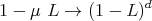(1)

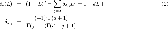
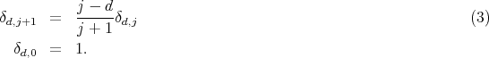
The new term (1 - L)^d is a fractional difference operator, defined through a Taylor expansion in the lag operator

(4)

The complete derivation for the GARCH(p,q) process is given in the original article Baillie et al. [1996].

The implementation of the FIGARCH process presents an important practical difficulty related to the cut-off of the fractional difference operator, as already pointed out first by Teyssière [1996] and Chung [1999]. These references have unfortunately not been published, but this problem is reviewed in details in Zumbach [2004]. In practice, the expansion of the fractional difference operator has to be cut-off at some upper limit j_max. The cut-off of the infinite sum implies that the identity δ_d(1) = 0 is not true anymore. This identity appears when taking the unconditional average of the above equation, in order to compute the mean volatility. For the differential operator with a finite cut-off, taking the average of the Eq. 4 and using E[r²] = E[σ eff²] = σ ∞², we obtain that ω fixes the mean volatility. Therefore, the affine FIGARCH process, or Aff-FIGARCH(1,d, 0), is defined by the equation

(5)

and the affine parameter σ∞ fixes the mean volatility (notice the confusion between the “Integrated” included in the process name and the linear/affine structure of the equation). The condition β < d enforces the positivity of σeff. A modification of this equation allows to define a linear FIGARCH process (see Zumbach [2004] and Zumbach [2012] for a complete discussion and more references on these processes).

The affine FIGARCH(1,d,0) process has three parameters (σ∞,β,d) (whereas the linear FIGARCH process has two parameters (β,d)). The parameters for the numerical simulations are:

• σ∞ = 0.11
• d = 0.25
• β = 0.10
• j_max = 32768 fixes the upper cut-off.

For this parameter values for d and j_max, we have δ_d(1) = 0.0607.

The innovations have a Student distribution with 3.3 degree of freedom. The simulation time corresponds to 50 years with a time increment δt = 3 minutes.

References