|
|
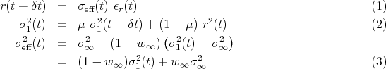
The GARCH model was introduced by Engle [1982], Engle and Bollerslev [1986], and used in countless subsequent papers. The equations are easier to understand in the formulation given in Zumbach [2004]
with the three parameters σ∞,w∞,τ, and with μ = exp(-δt ∕ τ). In this form, the GARCH(1,1) process is written with one “internal variable” σ1 that can be interpreted as a historical volatility measured by an exponential moving average at the time horizon τ. The variance for the next time step σeff2(t) is given by the mean term, plus the difference between the historical variance and the mean variance, weighted by 1 - w∞. In the second form, the next-step variance is a convex combination of the mean variance σ∞2 and the historical variance σ 12. With these equations, the three parameters have a direct interpretation in terms of the properties of the time series.Usually, the GARCH volatility equation is written in the equivalent form
 | (4) |
as it appears in the original article. The 3 parameters can be translated between both forms by using α0 = σ∞2(1 - μ)w ∞, α1 = (1 - w∞)(1 - μ) and β1 = μ. Although equivalent, the form (4) for the volatility equation has two drawbacks. First, it is less amenable to an intuitive understanding of the different terms. Second, the natural generalisation of Eq. 4 leads to the GARCH(p,q) form. Most studies find that GARCH(p,q) does not improve much over GARCH(1,1) for resonably small values of p and q. On the other hand, in the form 3, the GARCH equations lead to the introduction of more components σ1,σ2,σ3,..., with increasing time horizons τ1,τ2,τ3,.... With a few components, a large span of time intervals can be covered.
The process equations are affine for the variance, because the parameter σ∞2 (or α0) appears as an additive constant. This constant is important, as it fixes the mean level for the volatility.
The correlations for the GARCH(1,1) process can be computed analytically; they decay exponentially fast with a characteristic time τcorr = -δt ∕ ln(μcorr) with μcorr = α1 + β1 = μ + (1 -w∞)(1 -μ). The k-steps variance forecast formula can be expressed as
 = σ2∞ + μkc-or1r σ2eff(t) - σ2∞](description2x.png) | (5) |
showing explicitely the exponential mean reversion toward σ∞2 for large time intervals Δt.
The parameters for the simulations are
This corresponds to α1 = 0.00187, β1 = 0.99792 and a decay for the correlation of 10.0 day. The innovations have a Student distribution with 3.3 degree of freedom. The simulation time corresponds to 200 years with a time increment δt = 3 minutes.
R. F. Engle. Autoregressive conditional heteroskedasticity with estimates of the variance of U. K. inflation. Econometrica, 50:987–1008, January 1982.
Robert F. Engle and Tim Bollerslev. Modelling the persistence of conditional variances. Econometric Reviews, 5:1–50, 1986.
Gilles Zumbach. Volatility processes and volatility forecast with long memory. Quantitative Finance, 4:70–86, 2004.