| |
Normalized moments of the returnThe horizontal axis gives the time horizons of the returns, the vertical axis gives the normalized moments. |
|
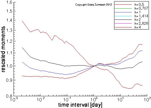 |
For a given exponent k, the moment E[|r[dt]|k]1/k
of the returns at various time interval dt. The exponent k takes the values 0.5, 1, 2 and 4 (the caption is incorrect!).
Each curve is multiplied by a constant such that the moment at dt = 1 day is equal to 1.
The graph scales are log-log, in order to search for power laws.
Remember that the definition of the returns already includes a factor (1y/dt)1/2, and therefore the usual random walk scaling is already discounted. Thanks to this convenient normalization, these moment scaling curves capture the deviations from a random walk. In roughly 2 decades from 0.1 to 10 day, the moments are nearly linear (in log-log scales), indicating a power law behavior (multifractal). The scaling for k < 2 (k > 2) show a positive (negative) slope, while the moment for k=2 is nearly flat (black line). Notice also the different behaviors at very short and very long time intervals. |
Normalized moments of the volatilityThe horizontal axis gives the time horizons of the volatility, the vertical axis gives the normalized moments. |
|
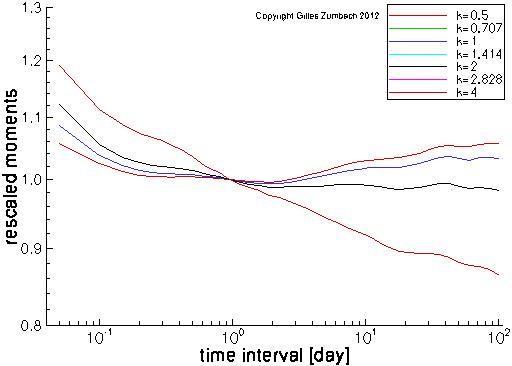 |
The moments computations (see above) for the volatility. Notice that the moments are not centered, namely the mean is not subtracted (contrary say to a standard deviation). |
Normalized moments of the volatility incrementThe horizontal axis gives the time horizons of the volatility increment, the vertical axis gives the normalized moments. |
|
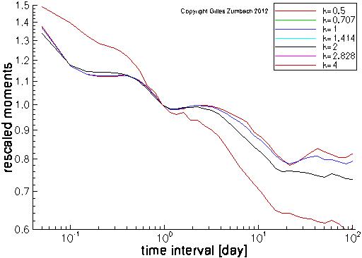 |
The moments computations (see above) for the volatility increment. |