Probability density function: description

Pdf for the return

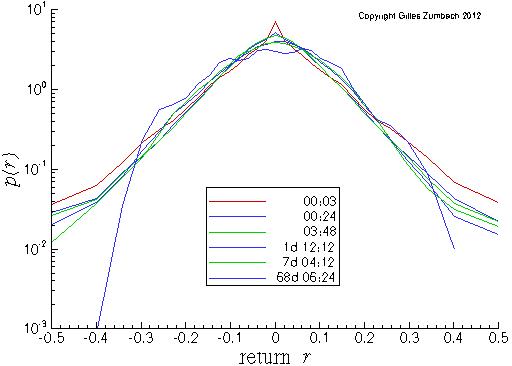
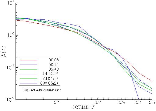
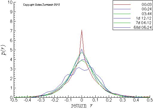Probability density for the return, in linear-logarithmic scales.

Probability density for the return, in log-log scales, for the positive returns.

Notice that the variance of the pdf is nearly stationary due to our definition of the return that removes the random walk scaling. With the increasing time horizons, the pdf converges (slowly) toward a Gaussian distribution due to the returns aggregation and the central limit theorem.

On the lin-log scales, notice at short time horizons the characteristic "tent shape" of the pdf. This shows that in a large domain of returns, the pdf is different from a Gaussian.

For very large returns, the expected shape of the pdf is to decays as a power law with exponent α+1. On a log-log scale (lowest graph), this should translate into a straight line ln(p(r)) ~ -(α+1)ln(|r|).

Pdf for the volatility

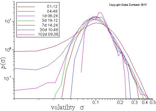
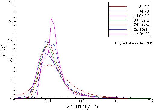Probability density for the volatility, in lin-log scales.

The slow modification of the pdf for an increasing time horizon is clear from the figure. Notice that the second moment of the pdf is nearly constant due to the annualization factor included in the volatility definition.

In the lin-log scales, the nearly quadratic shape close to the maximum is clearly observed. Yet, on the large volatility side, the shape is not well described by a quadratic shape. In this range, a linear description seems more appropriate.

Pdf for the volatility increment

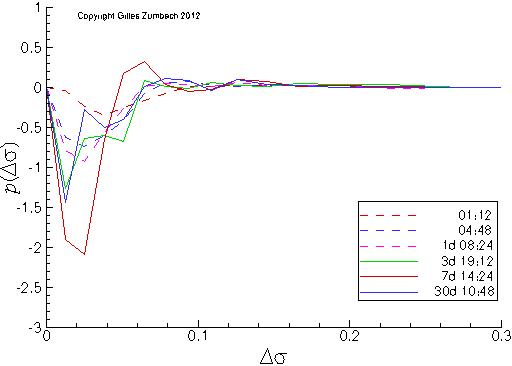
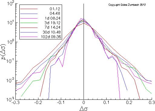Probability density asymmetry for the volatility increment.

The second graph measure the asymmetry between positive and negative volatility changes. A slight asymmetry between positive and negative volatility increments can be observed on empirical data. This shows that large volatility increases are more frequent than large decreases. This asymmetry is one measure of the non invariance under time reversal.